The Gaussian distribution

When you hear the term “bell curve” what you are actually listening to is a discussion of the “normal” or “Gaussian” distribution.

This is a probability density function (PDF) of the form:

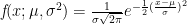
$\textit{f}(x; \mu,\sigma^2) = \frac{1}{\sigma\sqrt{2\pi}}e^{-\frac{1}{2}(\frac{x-\mu}{\sigma})^2}$

Here $\mu$ is the mean or expectation (peak) and $\sigma^2$ is the variance ( $\sigma$ is the standard deviation) and of course $e$ is Euler’s number (the base for natural logarithms).

But what does it all mean in a physical sense? Where does it come from?

Let’s look at variance first. This measures the spread of the function.

Take an example of a coin tossed four times. Assuming it is a fair coin then we should expect to get 2 heads. But, of course, the process is random so is likely to deviate from that. So variance being the square of deviation, what will that be?

There a $\frac{1}{2}^4 = \frac{1}{16}$ chance of four heads (or four tails), a $\frac{4}{16}$ chance of one head (or three heads, ie 1 tail) and a $\frac{6}{16}$ of 2 heads.

So the variance then becomes:

$\frac{1}{16}(0 - 2)^2 + \frac{4}{16}(1 - 2)^2 + \frac{6}{16}(2 - 2)^2 + \frac{4}{16}(3 - 2)^2 + \frac{1}{16}(4 - 2)^2$

Which comes out as 1.

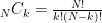
The normal distribution is a limiting case of the binomial distribution – which looks at success/fail type discrete variables (of course the coin example above is just such a case.) In the binomial distribution has a PDF of the form:

$f(k; N,p) = _NC_k p^kq^{(N-k)}$

Where $p$ is the probability of an event happening and $q = 1 - p$ is the probability of it not happening, and where $_NC_k$ is the binomial coefficient and can be spoken of as “N choose k” and is the number of ways of distributing $k$ successes from $N$ trials.

$_NC_k = \frac{N!}{k!(N-k)!}$

Consider the case where $N$ becomes large…

Here the change of success is p and the chance of failure is (1 – p), so the average result of each test is 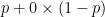$p + 0 \times (1 - p)$ , so the mean $\mu = Np$

The variance for each test is $p(1 - p)^2 + (1 - p)(0 - p)^2 = (1 -p)(p - p^2 + p^2) = p(1-p)$ so the total variance is $Np(1-p)$ .

Now, let’s look at the cumulative distribution function: this is the probability that the result will be less than or equal to $x$ , ie $P_r(X \leq x)$ .